- Cost planning
- Cost Analysis
- Cost management Techniques
- Externally oriented Cost Management Techniques
- Relevant costs
- Short term decisions
- Risk and Uncertainty
- Linear programming – graphical method
- Linear programming the simplex method
- Multi Product CVP Analysis
- Pricing decisions and Pricing strategies
- Budgetary Control
- Performance Evaluation
- Measuring performance in divisionalised businesses
- Transfer pricing
Risk and uncertainty in decision making
All businesses face risk. Risk is the variability of possible returns.
Risk management is important in a business. It is the process of understanding and managing the risks that an organisation is inevitably subject to.
Investment projects are long-term projects, often with a time scale of many years. When the cash flows for an investment project are estimated, the estimates might be incorrect. Estimates of cash flows might be wrong for two main reasons:
- Risk in the investment, and
- Uncertainty about the future
Risk – there are a number of possible outcomes and the probability of each outcome is known.
Uncertainty – there are a number of possible outcomes but the probability of each outcome is not known.
Methods of assessing risk and uncertainty
There are several methods of analysing and assessing risk and uncertainty. In particular:
- Sensitivity analysis
- Risk modelling and simulation
- Probability analysis and Expected values
- Maximax, maximin and minimax regret
- Decision Trees.
Risk attitudes
The selection criterion applied by the manager will often depend upon the manager’s attitude towards risk. It is common to recognise three different attitudes:
- Risk neutral –This person considers all possible outcomes and will select the strategy that maximises the expected value of benefit.
- Risk seeker – The decision maker is likely to select the strategy with the best possible outcomes, regardless of the likelihood that they will occur. This person will apply the maximax criterion
- Risk averse – This person will consider the worst outcome each time. They will apply the maximin criterion or the minimax regret approach.
Responding to risk and uncertainty
Risk is considered by using probability distribution, expected values, simulation, or CAPM (for adjusting discount rate for every project). Uncertainty is considered using the following measures:
- setting a minimum payback period for projects;
- increasing the discount rate to provide a more pessimistic measure of npv;
- making prudent / conservative estimates to assess the worst outcomes possible;
- performing scenario analysis to analyse the best and the worst possible situations and a range of outcomes; or
- using sensitivity analysis to measure the “margin of safety” on input data.
Probabilities and Expected values (EV)
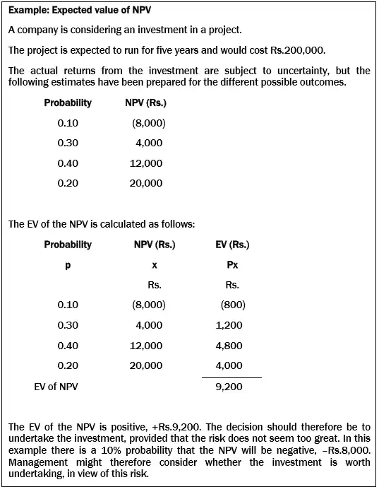
An expected value is a weighted average value, calculated using probability estimates of different possible outcomes. To calculate an expected value, the probability of each possible outcome is estimated, and the mean (average) outcome is calculated.
In other words, it is obtained by multiplying the value of each possible outcome (x), by the probability of that outcome (p), and summing the results.
Formula: Expected value
Expected value = Σpx
Where:
p = the probability of each outcome
x = the value of each outcome
When expected values are used to assess the risk in capital investment appraisal, x would be the NPV for each possible outcome, and the EV would be the expected value of the project net present value (the EV of the NPV).
*The basic decision rule is that an investment project should be undertaken if the expected value of its NPV is positive.
However, a project with a positive EV of NPV might not be undertaken if the risk involved seems too great in relation to the amount of the return expected.

Advantages and disadvantages of using expected values
Advantages
- Takes uncertainty into account by considering the probability of each possible outcome and using this information to calculate an expected value.
- The information is reduced to a single number resulting in easier decisions.
- Calculations are relatively simple.
Disadvantages
- The probabilities used are usually very subjective.
- The EV is merely a weighted average and therefore has little meaning for a one-off project.
- The EV gives no indication of the dispersion of possible outcomes about the EV, i.e. the risk.
- The EV may not correspond to any of the actual possible outcomes.
Data tables
Data tables are often produced using spreadsheet packages and show the effect of changing the values of variables.
A one-way or one-input data table shows the effect of a range of values of one variable. For example, it might show the effect on profit of a range of selling prices.
A two-way or two-input data table shows the results of combinations of different values of two key variables. The effect on contribution of combinations of various levels of demand and different selling prices would be shown in a two-way data table.
Any combination of variable values can therefore be changed and the effects monitored.
Data tables and probability
If a probability distribution can be applied to either or both of the variables in a data table, a revised table can be prepared to provide improved management information.
The maximin, maximax and minimax regret bases for decision making
When probabilities are not available, there are still tools available for incorporating uncertainty into decision making.
Maximin
The ‘play it safe‘ basis for decision making is referred to as the maximin basis. This is short for ‘maximise the minimum achievable profit‘. (It might also be called ‘minimax’ which is short for ‘minimise the maximum potential cost or loss’). Maximin decisions are taken by risk-averse decision makers.
Playing safe, and choosing the option with the least damaging results if events were to turn out badly.
The maximin rule involves selecting the alternative that maximises the minimum pay-off achievable. The investor would look at the worst possible outcome at each supply level, then selects the highest one of these. The decision maker therefore chooses the outcome which is guaranteed to minimise his losses. In the process, he loses out on the opportunity of making big profits.
The main weakness of the maximin basis for decision making is that it ignores the probabilities that various different outcomes might occur, and so in this respect, it is not as good as the EV basis for decision making.
Maximax
A basis for making decisions by looking for the best outcome is known as the maximax basis, short for ‘maximise the maximum achievable profit‘. (It can also be called the minimin cost rule – minimise the minimum costs or losses.) Maximax decisions are taken by risk-seeking decision makers.
The Minimax Regret rule
The ‘opportunity loss’ basis for decision making is known as minimax regret.
The minimax regret strategy is the one that minimises the maximum regret. It is useful for a risk-averse decision maker. Essentially, this is the technique for a ’sore loser’ who does not wish to make the wrong decision.
Minimax regret considers the extent to which we might come to regret an action we had chosen.

An alternative term for regret is opportunity loss. We may apply the rule by considering the maximum opportunity loss associated with each course of action and choosing the course which offers the smallest maximum. If we choose an action which turns out not to be the best in the actual circumstances, we have lost an opportunity to make the extra profit we could have made by choosing the best action.
Using the standard deviation to measure risk
Risk can be measured by the possible variations of outcomes around the expected value. One useful measure of such variations is the standard deviation of the expected value.

The decision maker can then weigh up the EV of each option against the risk (the standard deviation) that is associated with it.
Decision trees
Decision trees are diagrams which illustrate the choices and possible outcomes of a decision.
A Decision tree is ‘A pictorial method of showing a sequence of interrelated decisions and their expected outcomes. Decision trees can incorporate both the probabilities of, and values of, expected outcomes, and are used in decision-making.’
A decision tree is a diagrammatic representation of a decision problem, where all possible courses of action are represented, and every possible outcome of each course of action is shown. Decision trees should be used where a problem involves a series of decisions being made and several outcomes arise during the decision-making process.
A complex problem is broken down into smaller, easier-to-handle sections. Only relevant costs and revenues are considered, and that all cash is expressed in present value terms.
A decision tree is drawn from its “root” up to its “branches” and then, once drawn, analysed from its “branches” back to its “root”.
Exactly how does the use of a decision tree permit a clear and logical approach?
- All the possible choices that can be made are shown as branches on the tree.
- All the possible outcomes of each choice are shown as subsidiary branches on the tree.
Constructing a decision tree
Three-step method
Step 1 – Draw the tree from left to right showing appropriate decisions and events/outcomes.
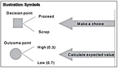
There are two different types of branching point in the tree:
- Decision points – as the name suggests this is a point where a decision is made
- Outcome points – an expected value is calculated here.
The following symbols are used for decision points and outcome points:

Square is used to represent a decision point (i.e. where a choice between different courses of action must be taken. A circle is used to represent a chance point. The branches coming away from a Circle with have probabilities attached to them. All probabilities should add up to ‘1’.
Step 2 – Evaluate the tree from right to left carrying out these two actions:
- Calculate an EV at each outcome point.
- Choose the best option at each decision point.
Step 3 – Recommend a course of action to management.
Evaluating the decision with a decision tree
Rollback analysis evaluates the EV of each decision option. You have to work from right to left and calculate EVs at each outcome point.
The EV of each decision option can be evaluated, using the decision tree to help with keeping the logic on track. The basic rules are as follows:
- We start on the right-hand side of the tree and work back towards the left-hand side and the current decision under consideration. This is sometimes known as the ‘rollback’ technique or ‘rollback analysis’.
- Working from right to left, we calculate the EV of revenue, cost, contribution or profit at each outcome point on the tree.
Evaluating decisions by using decision trees has a number of limitations:
- The time value of money may not be taken into account.
- Decision trees are not very suitable for use in complex situations.
- The outcome with the highest EV may have the greatest risks attached to it. Managers may be reluctant to take risks which may lead to losses.
- The probabilities associated with different branches of the ‘tree’ are likely to be estimates, and possibly unreliable or inaccurate.
The value of information
Perfect information is guaranteed to predict the future with 100% accuracy.
Perfect information removes all doubt and uncertainty from a decision, and enables managers to make decisions with complete confidence that they have selected the optimum course of action.
The forecast of the future outcome is always a correct prediction. If a firm can obtain a 100% accurate prediction they will always be able to undertake the most beneficial course of action for that prediction.
Imperfect information is better than no information at all, but could be wrong in its prediction of the future. The forecast is usually correct, but can be incorrect.
Imperfect information is not as valuable as perfect
The value of perfect information
The value of perfect information is the difference between the EV of profit with perfect information and the EV of profit without perfect information.

Step 1 – If we do not have perfect information and we must choose between two or more decision options, we would select the decision option which offers the highest EV of profit. This option will not be the best decision under all circumstances. There will be some probability that what was really the best option will not have been selected, given the way actual events turn out.
Step 2 – With perfect information, the best decision option will always be selected. The profits from the decision will depend on the future circumstances which are predicted by the information; nevertheless, the EV of profit with perfect information should be higher than the EV of profit without the information.
Step 3 – The value of perfect information is the difference between these two EVs.
The value of imperfect information
Perfect information is only rarely accessible. In fact, information sources such as market research or industry experts are usually subject to error. Market research findings, for example, are likely to be reasonably accurate – but they can still be wrong. Therefore, our analysis must extend to deal with imperfect information.
Sensitivity analysis
Sensitivity analysis is a useful but simple technique for assessing investment risk in a capital expenditure project when there is uncertainty about the estimates of future cash flows. It is recognised that estimates of cash flows could be inaccurate, or that events might occur that will make the estimates wrong.
The purpose of sensitivity analysis is to assess how the NPV of the project might be affected if cash flow estimates are worse than expected.
Sensitivity analysis takes each uncertain factor in turn, and calculates the change that would be necessary in that factor before the original decision is reversed. By using this technique, it is possible to establish which estimates (variables) are more critical than others in affecting a decision.
There are two main methods of carrying out sensitivity analysis on a capital expenditure project.
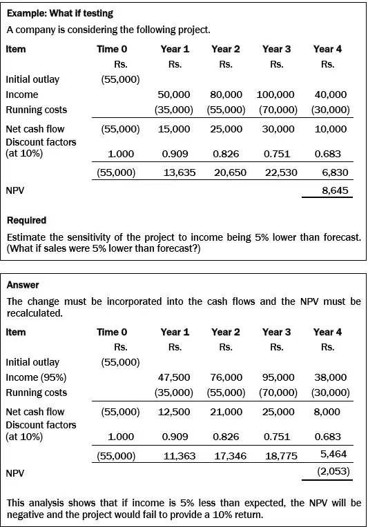
Method 1
Sensitivity analysis can be used to calculate the effect on the NPV of a given percentage reduction in benefits or a given percentage increase in costs. For example:
- What would the NPV of the project be if sales volumes were 10% below estimate?
- What would the NPV of the project be if annual running costs were 5% higher than estimate?
The percentage variation in the expected cash flows should be an amount that might reasonably occur, given the uncertainty in the cash flow estimates.
There are also forms of ‘stress testing’, similar to sensitivity analysis, that might be used to assess the investment risk. An assessment could be made to estimate the effects of:
- Of an unexpected event occurring in the future that would make the cash flow estimates for the project wrong; or
- The effect of a delay so that the expected cash inflows from the project occur later than planned.
This sort of analysis is sometimes called “what if?” analysis.
Method 2
Alternatively, sensitivity analysis can be used to calculate the percentage amount by which a cash flow could change before the project NPV changed. For example:
- By how much (in percentage terms) would sales volumes need to fall below the expected volumes, before the project NPV became negative?
- By how much (in percentage terms) would running costs need to exceed the expected amount before the NPV became negative?
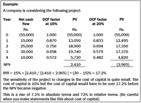
Estimating the sensitivity of a project to changes in the cost of capital
The sensitivity of the project to a change in the cost of capital can be found by calculating the project IRR. This can be compared with the company’s cost of capital.

Strengths of sensitivity analysis
- There is no complicated theory to understand.
- Information will be presented to management in a form which facilitates subjective judgement to decide the likelihood of the various possible outcomes considered.
- It identifies areas which are crucial to the success of the project. If the project is chosen, those areas can be carefully monitored.
Weaknesses of sensitivity analysis
- It assumes that changes to variables can be made independently, e.g. material prices will change independently of other variables. Simulation allows us to change more than one variable at a time.
- It only identifies how far a variable needs to change; it does not look at the probability of such a change.
- It provides information on the basis of which decisions can be made but it does not point to the correct decision directly.
Simulation models
Simulation is computer-based risk adjustment model which overcomes the problem of having a large number of possible outcomes and correlation between them.
Sensitivity analysis considers the effect of changing one variable at a time. Simulation improves on this by looking at the impact of many variables changing at the same time.
Using mathematical models, it produces a distribution of the possible outcomes from the project. The probability of different outcomes can then be calculated.
Steps in simulation
- Specify major variables, e.g.: market size, selling price, market growth rate, market share.
- Specify the relationships between variables to calculate an NPV.
- Simulate the environment:
- assign random numbers to represent the probability distribution for each variable
- draw a random number for each variable
- select the value of each variable corresponding with the selected random number and compute an NPV
- repeat the process many times to create a probability distribution of returns.
- The results of a simulation exercise will be a probability distribution of NPVs.
Advantages of simulation
The major advantages of simulation are as follows:
- it includes all possible outcomes in the decision-making process.
- it is a relatively easily understood technique.
- it has a wide variety of applications (inventory control, component replacement, corporate models, etc.).
Drawbacks of simulation
- models can become extremely complex and the time and costs involved in their construction can be more than is gained from the improved decisions.
- probability distributions may be difficult to formulate.

