- Cost planning
- Cost Analysis
- Cost management Techniques
- Externally oriented Cost Management Techniques
- Relevant costs
- Short term decisions
- Risk and Uncertainty
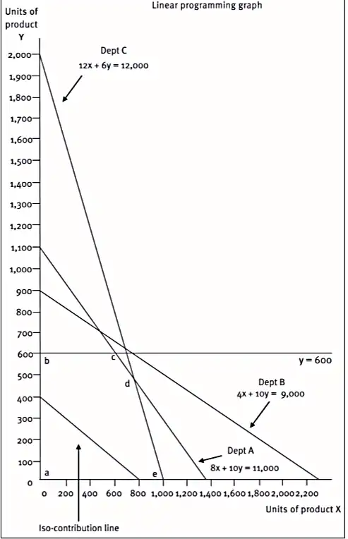
- Linear programming – graphical method
- Linear programming the simplex method
- Multi Product CVP Analysis
- Pricing decisions and Pricing strategies
- Budgetary Control
- Performance Evaluation
- Measuring performance in divisionalised businesses
- Transfer pricing
Linear programming: Graphical method
If faced with two or more limiting factors, then the situation is more complicated and linear programming techniques must be used (and the limiting factors are now called constraints). These linear programming notes are prepared by mindmaplab team and covering the linear programming introduction, theory, the first step in formulating a linear programming problem, the shadow price and slack concept with examples. These summary notes are actually the linear algebra full course for dummies. These linear programming questions and answers are also available in pdf too. We have also prepared the linear programming pdf version download.
Introduction
In decision making when faced with one limiting factor, we calculate the contribution per unit of the limiting factor and rank the products, allocating the scarce resource to the best product and then the next best product and so on until the resource is fully utilised.
If faced with two or more limiting factors, then the situation is more complicated and linear programming techniques must be used (and the limiting factors are now called constraints).
Firms face many constraints on their activity and plan accordingly:
- limited demand
- limited skilled labour and other production resources
- limited finance (‘capital rationing’).
Planning with one limiting factor
The usual objective in questions is to maximise profit. Given that fixed costs are unaffected by the production decision in the short run, the approach should be to maximise the contribution earned.
If there is one limiting factor, then the problem is best solved using key factor analysis:
Step 1: identify the scarce resource.
Step 2: calculate the contribution per unit for each product.
Step 3: calculate the contribution per unit of the scarce resource for each product.
Step 4: rank the products in order of the contribution per unit of the scarce resource.
Step 5: allocate resources using this ranking and answer the question.
Several limiting factors – linear programming
Where there are two or more resources in short supply which limit the organisation’s activities, then linear programming is required to find the solution.
linear programming is used to:
- maximise contribution and/or
- minimise costs
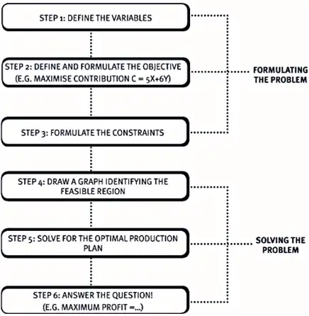
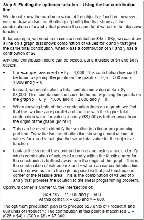
The steps involved in linear programming are as follows:
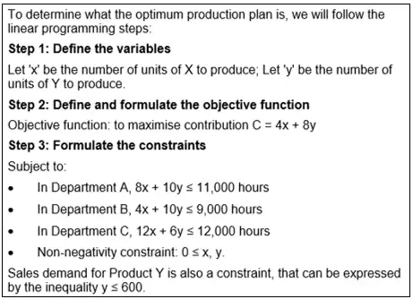
Example
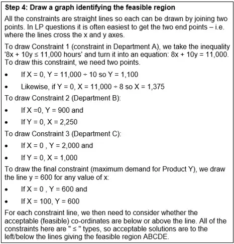
Solution

Limiting factor analysis – Assumptions
- There is a single quantifiable objective – e.g. maximise contribution. In reality there may be multiple objectives such as maximising return while simultaneously minimising risk.
- Each product always uses the same quantity of the scarce resource per unit. In reality this may not be the case. For example, learning effects may be enjoyed.
- The contribution per unit is constant. In reality this may not be the case:
- the selling price may have to be lowered to sell more
- there may be economies of scale, for example a discount for buying in bulk.
- Products are independent – in reality:
- customers may expect to buy both products together
- the products may be manufactured jointly together.
- The scenario is short term. This allows us to ignore fixed costs.
The assumptions apply to the analysis used when there is one limiting factor or if there are multiple limiting factors.
Shadow prices and slack
Slack
Slack refers to the amount of a constraint that is not used in the optimal solution to a linear programming problem.
Only non-limiting resources have slack. Limiting resources are fully utilised so never have any slack.
The amount of slack in any non-limiting resources is easily found by substituting the optimum product mix into the equation for that resource. This would show how much of that resource was needed for the optimum solution. This could then be compared to the amount of resource available to give the slack.
Shadow prices
The shadow price or dual price of a limiting factor is the increase in contribution created by the availability of one additional unit of the limiting factor at the original cost.
- The shadow price of a resource can be found by calculating the increase in value (usually extra contribution) which would be created by having available one additional unit of a limiting resource at its original cost.
- It therefore represents the maximum premium that the firm should be willing to pay for one extra unit of each constraint. This aspect is discussed in more detail below.
- Non-critical constraints will have zero shadow prices as slack exists already.
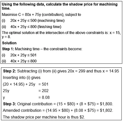
Calculating shadow prices
The simplest way to calculate shadow prices for a critical constraint is as follows:
Step 1: Take the equations of the straight lines that intersect at the optimal point. Add one unit to the constraint concerned, while leaving the other critical constraint unchanged.
Step 2: Use simultaneous equations to derive a new optimal solution.
Step 3: Calculate the revised optimal contribution and compare to the original contribution calculated. The increase is the shadow price.
