Tag: acca f2

IAS 38 Intangible Assets Study Text

Download the free IAS 38 Intangible Assets Study Text

October 8, 2019
IAS 37 Provisions, Contingent liabilities, Contingent assets Study Text

Download the free IAS 37 Provisions, Contingent liabilities, Contingent assets Study Text

October 8, 2019
IAS 36 Impairment of Assets Study Text

Download the free IAS 36 Impairment of Assets Study Text

October 8, 2019
High/Low and Linear Regression Analysis
Read More
High/Low and Linear Regression Analysis Overview

The total costs associated with a business are the SUM of fixed costs and variable costs i,e. the total cost is semi-variable in nature.
- Total costs can be divided into fixed costs /variable cost per unit of output.
  Formula for total costs:
Y=a+bx

where:
y= total cost in a period
a= the fixed costs in the period
b= the variable cost per unit of output or unit of activity
x= the number of output or the volume of activity in the period.

Constructing Total cost function

High/Low and Linear Regression Analysis

Methods for constructing Total cost function

The total cost function can be used to estimate costs associated with different levels of activities. Its useful for forecasting and decision making.

There are two methods for constructing the total cost function equation.
1. High/Low Analysis.
2. Linear Regression Analysis.
High/Low and Linear Regression Analysis

High/Low Analysis

High/Low analysis;

can be used to estimate fixed costs and variable costs per unit, whenever:
- figures available for total costs at two different level of output.
- it can be used that fixed costs are same and variable cost per unit is constant at both levels of activity.
- the different between the total costs at high level and low level of output is entirely variable cost.
The following circumstances are to be considered:

When No Change

Step 1: Take activity level and cost for:
- Highest level
- Lowest level
Step 2: Calculate variable cost per unit (b) as:

difference in total cost (highest minus lowest) divide by difference in no. of units (highest minus lowest).

Step 3: Now for fixed cost (a) put the variable cost per unit into one of the cost expressions (mostly high level).

Step 4: Construct total cost function for any activity level:
Total cost=a+bx

For Example:

Step 1
Highest level 7,000 (units) costs $38,800
Lowest level 4,500 (units) costs $30,400

Step 2: Difference
Therefore: variable cost per unit= 8400/2500 = $ 3.36

Step 3: Cost expressions: Total cost of 7,000 units

Fixed cost + variable cost= 38,800
Fixed cost + 7,000 x 3.36= 38,800
Fixed cost + 23,520= 38,800
Fixed cost=38,800–23,520=15,280

Step 4: Construct total cost function
Total cost=a+bx= 15,280+ 3.36x

A step change in fixed costs as money value And the amount is known

Step 1: Take activity level and cost for:
- Highest level
- Lowest level
Step 2: Make adjustment for the step in fixed cost:
- add the step in fixed cost in lower level; or
- deduct it from higher level
Now calculate variable cost per unit (b) as:

difference in total cost (highest minus lowest) divide by difference in no. of units (highest minus lowest).

Step 3: Now for fixed cost (a) put the variable cost per unit into one of the cost expressions (mostly high level).

Step 4: Construct total cost function for any activity level:
Total cost=a+bx

For Example:

Step 1

Highest level 7,000 (units) costs $ 38,800
Lowest level 4,500 (units) costs $ 30,400

Step 2: Make an adjustment for step in fixed cost. For example fixed costs increase by $3,000 when the activity level exceeds or equals 10,000 units.

Add the increase in cost in lowest activity level.

Therefore: variable cost per unit= 5400/2500 = $ 2.16

Step 3: Cost expressions: Total cost of 7,000 units
Fixed cost + variable cost= 38,800
Fixed cost + 7,000 x 2.16= 38,800
Fixed cost + 15,120= 38,800
Fixed cost=38,800–15,120=23,680

Step 4: Construct total cost function (un-adjusted levels):
- Above 10,000 units
Total cost=a+bx= 23,680+ 2.16x
- Below 10,000 units
Total cost=a+bx=(23,680-3,000)+2.16x
Total cost=a+bx= 20,680+2.16x

A step change in fixed costs is given as a Percentage amount

When there is a percentage change after a particular level, this means there are TWO levels which share same fixed cost.

Step 1: Take activity level and cost for (3 levels):
- Highest level
- Middle level
- Lowest level
Step 2: Choose the pair which is on the same side as the step.

Now calculate variable cost per unit (b) as:

difference in total cost divide by difference in no. of units.

Step 3: Now for fixed cost (a) put the variable cost per unit into one of the cost expressions (mostly high level).

Step 4: Construct total cost function for any activity level:

Total cost=a+bx

For Example:

Step 1
- Highest level 7,000 (units) costs $ 38,800
- Middle level 5,500 (units) costs $ 35,000
- Lowest level 4,500 (units) costs $ 30,400
Step 2: Pair with same percentage change. (assume a 10% increase in fixed costs when the activity level exceeds or equals 5,500 units)
- Highest level 7,000 (units) costs $ 38,800
- Middle level 5,500 (units) costs $ 35,000
Therefore: variable cost per unit= 3800/1500 = $ 2.53

Step 3: Cost expressions: Total cost of 7,000 units
Fixed cost + variable cost= 38,800
Fixed cost + 7,000 x 2.53= 38,800
Fixed cost + 17,710= 38,800
Fixed cost=38,800–17,710=21,090
Step 4: Construct total cost function (un-adjusted levels):
- Above 5,500 units
Total cost=a+bx= 21,090+ 2.53x
- Below 5,500 units
Total cost=a+bx=(21,090 x 100/110)+2.53x
Total cost=a+bx= 19,173+2.53x

A step change in variable costs (is given as a Percentage/money amount)
- When there is a step change in variable cost per unit as money value the same approach is needed as for a step change in fixed cost. (above)
- When the change in variable cost per unit is given as a percentage amount, then variable cost(s) per unit should be calculated for TWO levels:
- - variable cost per unit used above change ; and
  - variable cost per unit used below change.
High/Low and Linear Regression Analysis

Linear Regression Analysis

In summary, linear regression is a better technique then high/low analysis because;
- it is more reliable ; and
- it’s reliability can be measured.
Formula:

Line of best fit (y=a+bx) can be constructed by calculating values for “a” and “b” using:

a = ∑y – b∑x
n n
b= ∑xy – ∑x ∑y
n∑x2 – (∑x)2

where:

x = units
y = costs

Enter the values into the line of best fit (y=a+bx) and solve for b and then a .

The following table should be used for calculating values of “x” and “y”

Table

X Y X² XY
October 3, 2019
Introduction to Cost and Management Accounting
Read More
Classification of cost Overview:

Introduction to cost and management accounting
- Cost Accounting (classification of cost in cost accounting)
- - Cost Accounting involves the calculation and measurement of the resources used by a business in undertaking its various activities and is concerned with identifying cost of various things ( i.e. gathering data about cost of ‘products’ or ‘services’ and ‘cost of activities’).
- Management Accounting (cost classification in management accounting)
- - Management accounting includes cost accounting as one of its discipline but is wider in scope.
  - Management accounting provides information to management that helps it to run the business:
1. 1. it provides detailed financial information so that they plan and control the activities or operation for which they are responsible.
  2. this information helps managers to make other decisions i,e. planning, controlling and taking one-off decisions.
ALL organizations needs to know:
- how much it costs to make the products or provide its services.
- to make sure product/services is sold at a Profit.
- to control the entity.
- to measure to what extent it is achieving its objectives.
- to plan expenditure for future.
Introduction to Costs

Types of organizations

Manufacturing organizations

Types of costing systems they use:
- Basic manufacturing costing.
- Standard costing.
- Process costing.
- Job costing.
Service organizations

Types of costing systems they use:
- Standard costing.
- Job costing.
Key Terminology

Cost object

Any activity for which a separate measurement of costs is needed.

For Example
- cost of a department.
- cost of a project.
Cost unit

A unit of product or service for which costs are determined.

For Example
- cost of A car.
- cost of bread items.
- cost of An item.
Unit cost

The cost incurred by a company to produce + store + sell one unit of a particular product.
Unit cost includes ALL fixed and variable costs involved in production.

Types of Cost Classification

Classification of Cost by Type

Material costs

Material costs are the costs of any material items purchased with the intention of using them in fairly short term future.

For example
- Raw material that go into the production process.
- Cost of stationary, cartridges replacement.
Labour costs
- Labour costs are the employees remuneration costs paid by the entity and includes;
  - wages and salaries of part-time workers, bonuses, pension contribution etc.
Other expenses
- That costs which are not Material/ Labour costs and includes;
  - cost of services provided by external suppliers, telephone cost, rental costs, depreciation charges.
Classification of Cost by Function

Production costs

The costs that are incurred in manufacturing finished products up to the time goods are completed.

Includes:
- Material costs: of raw materials and components used in production.
- Labour costs: of all employees working for the manufacturing function.
  Other Expenses.
Non-Production costs

Includes:

Administrative costs

Cost of providing administrative services to entity, usually includes;
- Salaries to staff in administration.
- Cost of office space (rent)
- Other expense incurred for administration only.
Selling and Distribution costs

The costs incurred in marketing and selling good or services to customers and costs of delivering the goods.

The costs of after-sales services such as customer support services are usually included in these costs.

They usually include;
- Salaries to staff in selling and distribution.
- Advertising costs and other marketing costs
- Operating costs for delivery vehicles such as fuel costs and repairs.
- Other costs incurred for selling and distribution department.
Finance costs

These are the costs that are involved in financing the organization, e.g : Loan interest Bank O/D
- They are generally included in administration costs ; or
- alternatively finance costs might be excluded from cost accounting system.
* Some costs might be partly production, partly administration and selling & distribution e,g: salaries of managing director, building rental costs.
In such case costs are divided/ apportioned between function s on fair basis.

Cost classification by Nature

Direct costs

Costs that can be traced in FULL to a cost unit i,e. A direct cost can be attributed in its entirety to the cost of an item that is being produced.

The following are direct costs:

Direct Material

All the materials that are used directly in manufacturing a product or providing service.

Direct materials includes both raw materials and components.

Direct Labour

These are specific costs associated with labour-time spent directly on production of goods or services.

Direct Expenses

Expenses that can be attributed directly in full to a cost unit i,e. that have been incurred in full in making a unit of product/service .

* In manufacturing type organization direct expenses are not common.

Indirect costs (overheads)
- An indirect cost (overhead cost) is any cost that is not a direct costs.
- Indirect costs cannot be attributed directly and full to a cost unit.
- Indirect costs include production overheads and non-production overheads. Each of these might include the following:
Indirect Material

Indirect material are any materials that are used/consumed that cannot be attributed in full to the item. They are treated as overhead costs, maybe classified as production overheads, administration overheads, selling and distribution overheads.

For e.g. indirect production material includes some items of cleaning materials and any materials used by staff not engaged in production.

Indirect Labour

They mainly consists of the costs of indirect labour employees (who do not work directly on items that are produced) but may be necessary so that production takes place.

All employees in administration and marketing department including management are indirect labour.

Indirect Expenses

Many costs incurred cannot be directly linked to cost units e.g. Rental costs of factory.

In manufacturing company all costs of administration and selling & distribution are treated as indirect overheads.

Product Cost
- Product cost include the prime cost Plus production overhead.
- Product cost are associated with goods that are produced or purchased for resale.
- They are inventory and only expensed out when sold.
Period Cost
- The costs that do not contribute towards the value of inventory.
- These are expensed in the period in which they occur.
Cost Behavior

Cost Behavior definition:
- Cost behavior refers to the way in which costs changes as volume of the activity changes.
- As a general rule, total costs are expected to increase as volume of activity rises.
- Understanding of cost behavior helps to;
- - forecast/plan what costs ought to be.
  - compare actual cost with budgeted.
Cost Classification by behaviour;

Fixed costs

These costs remain fixed/same in total during a period no matter how many units are produced and regardless the volume or scale of a activity.

However, the cost per unit falls because the cost is being spread over a greater number of units.

Semi-Variable cost
- A semi-variable cost is a cost that is partly fixed and partly variable.
- It is often assumed that total costs of an activity are mixed.
Stepped cost
- A cost which is fixed within a limited range of activity and goes up or down in steps when the volume of activity rises above or falls below certain levels.
Variable costs
- These costs increase usually by the same amount for each additional unit of product or service provided.
- The variable cost of a cost unit is also called marginal cost of unit.
- This means that total variable costs increase in direct proportion to the volume of output or activity.
- The cost per unit remains fixed . However, total cost increase as more units are made.
October 3, 2019
Time Value of Money (TVM) – formula with examples
Read More
Time Value of Money Overview

Discounted cash flow analysis
- It is a technique for evaluating the proposed investments to decide whether thy are financially worthwhile.
- The expected future cash flows (inflows/outflows) from the investment are all converted to a present value by discounting them at the cost of capital ‘r’
- Taking into account the concept of relevant cost.
- It is usually assumed that cash flow early during a year should be treated as a cash flow as at the end of the previous year.
Present value Formulas

Discount factor = 1/(1+r)n

where
r = cost of capital
n = number of periods

Annuity factor = ( 1 – (1+r)-n /r)

Discounted Cash Flow

Time Value of Money

Methods of Discounted Cash Flow

Net Present value (NPV)
- In Net present value (NPV) analysis, all future cash flows from a project are converted into a present value.
- NPV is the difference between present value of all costs incurred and present value of all benefits received.
Approach
1. List all cash flows from the project (initial investments, future cash inflows/outflows).
2. Discount these cash flows to present value using ‘cost of capital’ as discount rate.
3. If present value of Benefits exceeds the present value of costs, the NPV is positive and if present value of benefits is less, then NPV is negative.
- A project is worthwhile if NPV is positive.
- The project commences at time ‘0’ where the cash flows are already at present value.
- Changes in working capital included as cash flows. An increase usually at the beginning of the project in time ‘0’ is a cash outflow and reduction is a cash inflow.
Internal Rate of Return (IRR)
- It is the discounted rate of return on investment.
- It is the average annual investment return from the project.
- The NPV of the projected cash flows is ‘zero‘ when those cash flows are discounted at IRR.
- A company might establish the minimum rate of return that it wants to earn on an investment:
- - If a project’s IRR is equal or higher than minimum acceptable rate of return, it should be undertaken.
  - If IRR is lower than the minimum required return, it should be rejected.
- The following step are involved for calculation of a reliable Internal rate of return (IRR):
1. 1. Calculate NPV of the project at TWO different rates. One of the NPV should be positive and the other should be negative.
  2. Put the NPVs in the formula:
Discounted Cash Flow and Inflation

Time Value of Money

Methods of incorporating Inflation

Real cash flows
- The cash flows expressed in today’s price terms.
- They ignore the expectations of inflation.
- In order to incorporate real cash flows in NPV calculation, real cash flows should be discounted at the real cost of capital.
The following steps are involved:
- Calculate real discount rate
= money cost of capital – 1
inflation rate
- Calculate net cash flows at today’s prices.
- Discount them using real discount rate.
Money cash flows

This is the most common method used.
- Money (nominal) cash flows are cash flows that include expected inflation.
- Money cash flows should be discounted at the money cost of capital.
The following steps are involved:
1. Calculate net cash flows at today’s price.
2. Make adjustment for inflation (by doing this they will be converted into money cash flows).
3. Use money cost of capital as discount rate.
*Both approaches give same solution, with a difference of rounding off.
October 2, 2019
Relevant costing and Decision Making Techniques
Read more
Relevant costing and Decision Making Techniques Overview

Definitions:

Relevant cost
- A relevant cost is a future cash flow that will occur as a direct consequence of making a particular decision.
- They cannot include any cost occurred in past.
- Costs that occur whether or not a particular decision is taken are not relevant costs.
- Relevant costs are cash flows. Notional costs such as depreciation, interest costs and absorbed fixed cost are not relevant cost.
Incremental cost
- Any incremental cost, if a particular decision is taken, results in cash flow are relevant cost.
Differential cost
- A differential cost is an amount by which future costs will be higher or lower. A differential cost is a relevant cost.
Avoidable and unavoidable cost
- Avoidable costs are relevant costs
- Unavoidable costs are not relevant.
Committed costs
- Committed costs are unavoidable costs, therefore not relevant for decision making.
Sink costs
- Cost that are already incurred/or committed by an earlier decision. Such costs are not relevant costs.
Opportunity costs
- The relevant cost is the benefit that would be lost by switching to other work.
Identifying Relevant costs

Relevant costs of:

Materials

When Material currently in inventory

Are material in regular use?
- Yes
The relevant cost is the current Replacement cost.
- No
The relevant cost is the current opportunity cost.
Opportunity cost is higher of;
1. Net disposal/sales value/scrap value or;
2. Net benefit from alternative use.
When Material not currently in inventory

In this case the relevant cost is simply the purchase value.

Labour
- If the cost of labour is a variable cost and labour is not in restricted supply: The relevant cost is its variable cost.
- If labour is a fixed cost and there is spare labour time available: The relevant cost of using labour is ‘zero‘. The spare time would otherwise be paid for idle time.
- If labour is in unlimited supply: Relevant cost includes the opportunity cost of using the labour time for the decision instead of next most profitable way.
Overheads
- Normal rules of relevant costs are applied i,e Relevant costs are future cash flows.
- Fixed overheads absorption rate are irrelevant. However the variable overhead hourly rate is treated as relevant cost.
- The only overhead fixed costs that are relevant costs are the extra cash spending.
Decision Making Techniques

Types of Decisions
- The concept of relevant costs can be applied for both ‘long term’ and ‘short term’ decisions.
- The application is same for both types of decisions except for long term decisions ‘time value of money’ should be considered.
Such Types of Decisions are:

Limiting Factor Decisions
- Limiting factor are the factors that ‘restricts‘ operational capabilities, sales demand is normally the factor that sets a limit on volume of production. However the availability of scarce resources such as Direct material, skilled labour or machine capacity could be the limiting factor.
- If the company makes just one product and a production resource is in limited supply, profit is maximized by making as many units of product as possible with limited resources.
- However, if the company produces more than one product with same scarce resources then a budgeting problem is to decide how many of each product to make and sell in order to maximize Profit. In Such case select products for manufacture and sale according to the contribution per unit. The following steps are involved:
1. Calculate the contribution per unit of each good produced.
2. Identify scarce resources (e,g labour hours).
3. Calculate the amount of scarce resources used by each good produced (e,g ‘X’ no. of labour hours)
4. Now divide the contribution earned by each good by scarce resources used by that good to give the contribution per unit of scarce resources for that good.
5. Rank each good in order of contribution per unit per scarce resources (highest contribution is ranked 1st).
6. Construct a production plan based on ranking.
Assumptions of limiting factors:
- Profit is maximized by maximizing contribution.
- Variable costs are only the relevant costs.
- Fixed cost will be the same whatever decision is taken. Therefore are not relevant.
One-off contractual decisions
- The contract where the Job is once only and will not be repeated in future.
- The one-off contract is under taken if extra revenue is higher than relevant costs.
- The decision is to whether agree to do the Job at a Price offered by customer or decide a selling price (base on relevant costs).
- Profit = Revenue – Relevant cost
- One-off contract decisions might occur when a company has spare capacity and an opportunity arises to earn some extra profit.
Make-or-Buy decisions
- A decision whether: to make an item internally or buy it externally. The decision should be based on relevant cost, the preferred option from a financial view point is the one with the lowest relevant costs.
- A financial assessment of a make or buy decision involves a comparison of:
- - cost that would be saved; and
  - incremental cost of outsourcing
- A situation may arises where entity is operating in full capacity, in order to overcome some restrictions on its output and sales, the entity may outsource some products.
- The decision is about which item to outsource and which to retain in-house.
- The profit maximizing decision is to which items to outsource.
- Those items are outsource where cost of outsourcing is least.
- To identify the Least-cost of outsourcing, it is necessary to compare:
- - additional cost of outsourcing; with
  - amount of resources need to make product in-house.
Make-or-buy decision non-financial considerations

Non-financial considerations will often be relevant to make-or-buy decision:
- When work is outsourced, the entity loses some control over the work. It will rely on the external supplier. There may be some risk that external supplier will:
- - provide a lower quality.
  - fail to meet delivery on said dates.
- The entity will lose some flexibility. If it needs to increase or reduce supply of the outsourced item at short notice.
- Redundancy of employees may occur as a consequence of outsourcing affecting relations between management and other employees.
Shut-down Decisions
- A shutdown decision is whether or not to shut down a part of the operations of a company.
- From a financial view an operation should be shutdown if the benefits of shutdown exceeds relevant costs.
Example of such costs
- Fixed costs may be saved, Employee redundancy cost.
Joint Product further processing decisions
- Joint products are product manufactured from a common process.
- The entity has a choice whether:
1. 1. selling joint product as soon as it is output; or
  2. processing it further before selling (at a higher price).
- This is a short-term decision and financial assessment should be made using relevant cost and revenues. The financial assessment should compares:
1. 1. Revenue (less) selling cost from joint product as soon as it is output.
  2. The revenue that will be obtained if Joint product is processed further (less) incremental cost of further processing.
October 2, 2019
Process Costing – steps with examples
Read more
Process Costing Overview
- Process costing is used when output is produced in a continuous process system and it is difficult to separate individual units of output.
- It is not possible to have abnormal loss and gain on the same account in the same period.
- Whatever the complications, the task that sits at the heart of process costing is always to allocate the costs collected on the debit side of the account to possible output on the credit side.
- Basically we will need to:
1. Identify the losses and output units.
2. Calculate the cost of good output, losses and WIP.
3. Use the costs calculated to assign to good output, losses and WIP (i,e units x cost)
4. Complete the process account.
Losses

Total Losses

Normal Losses
- It is the expected loss in processing and is usually expressed as a percentage of input units of materials.
- It is inherent in the process and is unavoidable.
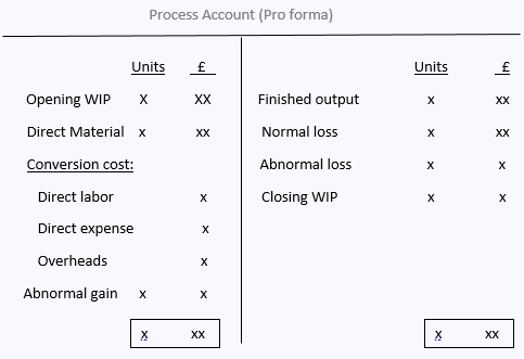
Normal loss = material input – expected output

Normal loss with recovery/scrap value
- when losses in a process has scrap value then the company is able to recover some of input costs.
- The scrap value reduces overall cost of the process.
- In process account Normal loss is measured at scrap value.
Cost of output = Total process cost – scrap value
Expected output
Expected output = material input – normal loss

Normal loss without recovery/scrap value
- The cost of lost units is part of the cost of obtaining the good output.
- All of the cost should be assigned to the good output and none to the normal loss.
- It is given a NIL value when the loss has no scrap value.
- Disposal cost of normal loss is an addition to costs to the process and debited to process account. It is added to total process costs when calculating cost of good output.
Cost of output = Total process cost – scrap value
Expected output

Abnormal Losses
- The difference between total actual loss and normal loss is ‘abnormal loss’.
- Abnormal loss is not expected and given a cost.
- If it is assumed that losses occur at the end of process, units of abnormal loss are costed exactly as finished output units i,e cost per units of abnormal loss is same as cost of units of good output
Cost of output = Total process cost – scrap value
Expected output
- Abnormal loss is treated as an expense and charged in Income Statement.
Abnormal Gain

Abnormal Gain
- The difference between normal loss and the total actual loss, where the actual loss is less then normal loss.
Abnormal Gain = Normal loss – Actual loss
- Abnormal gain is a benefit rather than a cost.
- Abnormal gain is an adjustment the increases the profit for the period.
- It is recorded as a debit entry.
Abnormal Gain where loss has NO scrap value
- If it is assumed that all losses occur at the end of the process, the cost per unit of finished output and the value/cost of abnormal gain is calculated as the cost per expected unit of output.
- The cost per unit of abnormal gain is therefore the same as the cost of units of good output.
Cost of output = Total process cost – scrap value
Expected output

Abnormal Gain where loss has a scrap value
- When loss has a scrap value, the value of abnormal gain is actually less than the amount shown in the process account. As the balance on the abnormal gain account is netted off by the scrap value.
- The balance is transferred as a net benefit to the Income Statement.
Losses and Gains at different stages in the Process
- If it is assumed that losses occur at the end of the production process, units of abnormal loss or gain are given a cost or value as if they are fully completed units and so one equivalent unit each. But is no relevant for normal loss.
- However, if losses occur at a different stage in the process, this assumption of differing degrees of completion is used for direct material and conversion, instead the concept of equivalent unit is used to decide the cost of abnormal loss/gain.
Valuation

of Abnormal loss

When loss occurs part-way through a process, the cost of any abnormal loss is calculated:
- establishing the equivalent units of direct material and conversion costs for loss.
- calculating a cost per equivalent units.
- using the calculations of equivalent units and cost per equivalent units to obtain a cost for finished output and abnormal loss in period.
of Abnormal Gain

The same principles apply to the valuation of abnormal gain, where the gain occur part-way through the process as abnormal loss.

However there is one important difference, equivalent units of abnormal gain are given a Negative value and subtracted from the total equivalent units of output in the period.

Work in Progress Balance

Work in Progress Balance

Opening Work in Progress
- When there is opening WIP there are two types of costs on the debit side. The opening WIP and the cost incurred in current period.
- The issue is whether these type of costs should be treated together or separately. The question is addressed in the accounting policy adopted for opening WIP. The following are two policies adopted:
weighted average cost method
- When this is used the assumption is that all units produced during the period and all units in closing inventory should be valued at the same cost per equivalent units for materials and conversion i,e an average cost per equivalent unit is calculated for all units of output and closing inventory.
- A three stage calculation is used:
1. Prepare statement of equivalent units.
2. Prepare statement of cost per unit equivalent units
3. Prepare statement of evaluation.
FIFO cost method
- Based on the assumption that the opening WIP are the first units completed. It is necessary to calculate the number of equivalent units for:
- - WIP opening
  - Finished output
  - WIP closing
- The three stage calculation is used for equivalent units and cost allocation.
- The three stage calculation is similar as weighted average with the exception that in statement of evaluation finished output consists of:
- - The finished cost of opening WIP is the sum of: costs in opening WIP value at start of period PLUS cost incurred in current period to complete these units PLUS the cost of finished output started and finished in the period.
Closing Work in Progress
- Closing WIP means some units have been started and finished in the year and others have been started but not finished.
- It stands to reason that cost/value of an unfinished unit is less than the cost of a completed unit. The cost of the process must be shared between finished output and unfinished WIP. In order to do this the concept of equivalent is used.
- A three stage calculation:
1. Prepare statement of equivalent units.
2. Prepare statement of cost per unit equivalent units.
3. Prepare statement of evaluation.
Joint Products and By-Products

Process costing

Joint Products and By-Products

Joint Products

Joint products are two or more products generated simultaneously, by a singe manufacturing process, using common input, and being substantially equal in value.

Apportioning common processing costs
- The costs of the common process that produces the Joint products are common costs. They must be apportioned between Joint products.
One of the following methods is used:

Units Basis

Common costs are apportioned on basis of total number of units produced.

Sales value at split-off point

Common costs are apportioned on basis of the sales value of Joint product produced when they are separated in process.

Net realizable value

Common costs are apportioned on basis of the sales value of Joint product produced when they are separated in process.

By-Products

When two or more different products are produced. Any product that does not have a substantial sales value and relatively minor in quantity is called a by-product.

Treatment of By-Product

Any of following method is used:
- Adding it to revenue from sales. No cost is allocated to by-product.
- As other income. No cost is allocated to by-product.
- As a deduction from Joint process costs (the most common method used).
- - By-product is measured at scrap value, similar to normal loss.
October 2, 2019
Variances – Formulas with examples
Read more
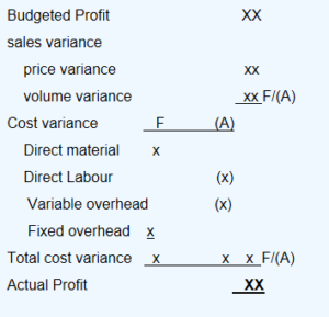
Variances analysis Overview
- Difference between expected results and actual results are known as variances. Variances can be either Favorable (F) or Adverse (A).
- Variances are calculated by comparing actual results with flexed budget.
- Variances are reported in a statement for the accounting period that reconciles the budgeted profit with the actual profit for the period. The statement is known as an Operating statement.
- - Large adverse variances indicate poor performance
  - Large favorable variance indicate unexpected good performance.
Variances: A summary

Variances

Sales variances
- Sales variances are not recorded in a standard costing system of cost accounts/cost ledger.
- Included in variance report (operating statement) to management.
- They help to reconcile the actual profit with budgeted profit.
Types
1. Sales Price Variance
2. Sales Volume Variance
Cost Variances
- The method of calculating cost variances is similar for all variable production cost items (Direct material, Direct labour, Production overheads). A different method of calculating fixed production overhead.
- The total cost variance is the difference between actual and standard variable cost of production. However, total cost variance is not usually calculated. Instead it is calculated in TWO parts.
- Cost variances are adjustments to the profit in an accounting period:
- - Favorable variances INCREASE profit.
  - Adverse variances REDUCES profit.
Types

Direct cost Variance
- Direct material Variance
- Direct labour Variance
Indirect cost/overhead Variance
- Variable Production overhead Variance
- Fixed Production overhead Variance
Cost Variances

Direct material Variance

Total cost variance

The total direct material cost variance is the difference between actual material cost of actual units and the standard material cost of actual costs.

Standard material cost of actual production:
- Actual units produced x standard kg/units x standard price per kg/unit XX
Actual material cost of actual production:
- Actual units produced x Actual kg/units x Actual price per kg/unit XX
Price variance

A price variance measures the difference between the actual paid for material and the price that should have been paid.

Standard material cost of actual production:
- Actual Kgs purchased x standard price per kg/unit XX
Actual material cost of actual production:
- Actual Kgs purchased x Actual price per kg/unit XX
Usage variance
- A usage variance measures the difference between material that were used in production and materials that should have been used.
- The difference is measured as a quantity of materials. This is converted into a money value at the standard price for material.
= Standard Price (standard quantity – Actual quantity)

Usage variance is further analysed into:

1. Material Mix Variance

= Standard Price (Total actual quantity x standard mix) – (Total actual quantity at actual mix)

2. Yield Variance

= Standard cost (standard output at actual mix) – (Actual output of actual mix)

Direct labour Variance

Direct labour Variance

Total cost variance

The total direct labour cost variance is the difference between actual labour cost in producing units and the standard labour cost of producing those actual costs.

Standard actual cost of actual production:
- Actual units produced x standard hrs/units x standard rate per hour XX
Actual labour cost of actual production:
- Actual units produced x Actual hours per unit x Actual rate per hour (XX)
Rate Variance

A rate variance measures the difference between the actual wage rate paid to per labour hour and the rate that should have been paid.

It looks at the hours paid.
Calculated as:

= Actual hrs (standard rate – actual rate)

Efficiency Variance

An efficiency variance or productivity variance measures the difference between the time taken to make the production output and the time that should have been taken.

The difference is measured in hours and converted into a money value at the standard direct labour rate per hour.

It looks at the hours worked.

Calculated as:

= Standard rate per unit (standard hrs – actual hrs)

Idle time variance
- Idle time variance is a part of Efficiency variance.
- Sometimes idle time might be a feature of a production process, in that case the expected idle time might be built into the standard cost. If idle time is not built into the standard cost, the idle time variance is always adverse.
- Calculating the idle time variance will affect the calculation of the direct labour efficiency variance, if idle time occurs but is not recorded.
Idle time not part of standard cost

If idle time is not included in standard cost any idle time is unexpected and leads to an adverse variance.

Idle time included in standard cost

Include idle time as a separate element of standard cost so that standard cost of idle time is a part of total standard cost per unit ; or

Allow for a standard amount of idle time in standard hours per unit for each product. The standard hours per unit therefore include an allowance for expected idle time.

Variable Production Overhead variance

Variable Production Overhead variance

Total cost variance

Standard Cost
- Actual units x standard hours per unit x standard rate per hour X
Actual Cost
- Actual variable production overheads (X)
Expenditure variance

It is the difference between actual variable overhead spending in hours worked and what the spending should have been (standard rate)

Similar to a material price variance or a labour rate variance.

= Actual hours (standard rate – actual rate)

Efficiency variance

The variable overhead efficiency variance in hours is same as the labour efficiency variance in hours (excluding any idle time variance) and is calculated in a very similar way.

= Standard Rate (standard hour – actual hours)

Fixed Production Overhead variance

Fixed Production Overhead variance
- The amount of fixed production overheads represents production overheads absorbed into production cost at a standard cost per unit produced.
- The amount of fixed production overhead absorption rate is a function of the budgeted fixed production overhead expenditure and volume.
- The total fixed overhead variance is the total amount of under-absorbed or over-absorbed overheads.
Total cost variance

Budgeted Cost
- Actual units produced x F.OH rate X
Actual Cost
- Actual overheads incurred (X)
Expenditure variance

= Budgeted F.OH – Actual F.OH

Volume variance

Can be measured in either units of output or standard hours.

= Standard cost (Budgeted Production – Actual Production)

Volume variance is further analyzed into:

Efficiency variance

Same as labour and variable production overhead variance in hours (worked/allowed).

= Standard Rate (standard hours – actual hours)

Capacity variance

= Standard Rate (budgeted hour – actual hour)
Excluding idle time.

Sales Variance

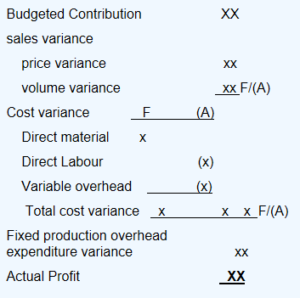
Sales variance

Total sales variance

= Budgeted contribution – Actual Contribution

Price variance

= Actual units sold (budgeted contribution – actual contribution)

Volume variance/ Volume profit variance

= Standard contribution or profit per unit (budgeted volume – Actual volume)

Reconciliation of Budgeted and Actual Profit (OPERATING STATEMENT)
- Operating statement reconciles profit between Budgeted and Actual by reporting all the variances to management , showing the difference between Budgeted and actual profit. Arises because of sales variance and cost variance.
Format

Absorption costing
- Absorption costing operating statement begins with Budgeted Profit.
- The sales variance are Next.
- The cost variance are listed next sales variance.
- Separate columns for the favorable and adverse variance.
- - Adverse — Reduces profit
  - Favorable — Add to profit.
- Actual profit is shown as final figure.
Marginal costing
- Marginal costing operating statement – All the formatting is same as absorption costing format expect there is no fixed production overhead volume variance.
- Where as fixed cost expenditure variance are presented in a separate part of the statement.
- In marginal costing ‘Budgeted contribution’ is used instead of ‘Budgeted profit’.
October 2, 2019
Standard Costing – Types, Meaning and Objectives
Read more
Standard Costing Overview

Standard cost
- A standard cost is an estimated/predetermined unit cost of performing an operation or producing a good or services under normal conditions.
- The predetermined unit cost (standard cost) is based on expected direct materials quantities and expected direct labour time and priced at a predetermined rate per unit of direct materials and rate per direct labour hour and rate per hour of overhead.
- Overheads are normally absorbed at direct labour hour.
Standard costing
- Standard costing is a control technique that report variances by comparing actual cost to pre-set standards. Standard costing may use; absorption or marginal costing.
Types of Standard

Types of Standard

Ideal Standard

This assumes perfect operating conditions.

No allowance for wastage is made.

Unlikely to be achieved.
Reported variance is always adverse

Attainable Standard

This assumes efficient but not perfect operating conditions.

An allowance for wastage is made.

Attainable targets.

Current Standard

These are based on current working conditions.

Includes an allowance for the expected wastage or idle time.

Basic Standard

This remains unchanged over a long period of time.

Variances are calculated by comparing actual results with basic standard.

Idle Time
- Idle time are the hours for which the direct labour employees are paid for no work.
- Idle time is recorded and the hours lost due to idle time are measured.
Methods of including idle time in standard costs

As a separate elements of standard cost
- Standard of idle time is a part of Total standard cost per unit.
Allowance for expected idle time
- Allows for a standard amount (pre-set amount) of idle time in standard hours per unit of each product, therefore including an allowance for expected idle time.
Budget
- Budget: A budget is a formal plan (for a specified time period) covering all the activities of the entity.
- It is a statement of what the entity is going to strive to achieve in future.
- Standard costing is a component of budgeting.
- Standard costs for a unit are often set out in record called a standard cost card.
Types of Budget

Fixed Budget
- It is the original budget prepared at the beginning of a budget period.
- It is prepared for a specific volume of output and sales activity.
- It is the master plan for the financial year that company tries to achieve.
- Variances are NOT calculated by comparing actual results to fixed budget directly.
Flexed Budget
- It is drawn-up at the end of the period.
- It is based on the actual levels of activity and standard revenue and standard costs.
- This shows the amount that the company would have received for the actual number of units sold if they had been sold at the budgeted revenue per item.
- Variances are calculated by comparing actual results with flexed budget.
October 2, 2019